What are Convolutional Neural Networks?
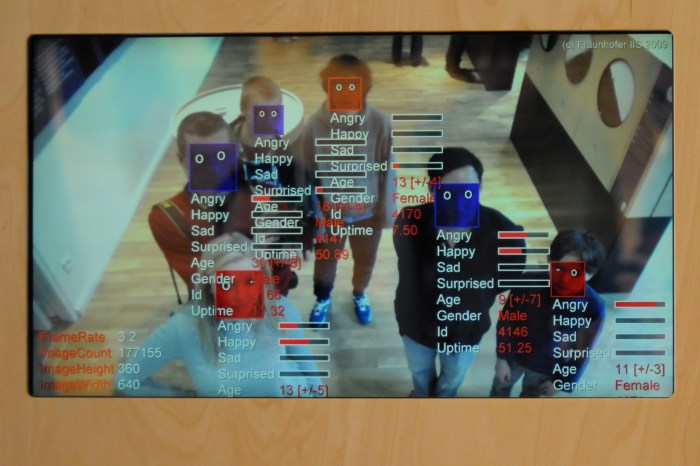
Convolutional Neural Networks (CNNs) categorize images and are responsible for the image recognition technologies behind self-driving cars, Facebook image tagging, emotional interpretation, and so forth. The trained model takes in images and returns identification judgments: is it a stop sign? is this Lebron James? is this a happy person or a sad armadillo? etc.
Taking their cues from the way in which humans classify images, CNNs aim to identify features that help distinguish what an image might and might not contain. Presence of particular shapes may indicate a nose, which suggest a face, which adds a piece to the puzzle of classifying what species/gender/individual the photo may be of – even down to names of specific people in photos.
Convolution Operation
The first step in a CNN is Convolution. This involves passing a feature detection grid (also referred to as a filter) across the input image in a systematic manner to generate a feature map, also known as the Convolved Feature or the Activation Map. (The step size when moving this detection grid is referred to as the Stride.) This is repeated with many feature maps to create our first Convolutional Layer.
While this process was comprehensible enough as conceptually intuitive, the details of feature detection filters comes to live with visual analogies. My mind was blown when Kirill ran through the examples of filters (most of which are not applicable to feature detection in our case) side-by-side with their actual detection grids on this gimp documentation page. We can see clearly that the features are distorted/enhanced in specific ways that correspond with targeted values in the filter grid, but that the spatial relationships between pixels are maintained. Not only did this visual exercise solidify the connection between filter vocabulary, process, and outcome, but it also made sense! For now.
On top of this first Convolutional Layer, we apply the rectifier function to create the ReLU (Rectified Linear Unit) Layer to increase nonlinearity. Visualizing this does not clarify the benefit of this step quite as well because it is a much more mathematical benefit than is physically apparent. Further reading is available to clarify and I am eager to delve into the mathematics on this as time permits.
Max Pooling
The process of pooling, also called downsampling, contributes to the spatial invariance, which reduces overfitting or reliance on rigid relationships between pixels. We can choose Max, Min, Sum, or Mean Pooling but will choose to focus on Max Pooling for the CNN we will build to approach our business problem.
An example of this layer, as well as surrounding layers, is available in this 2D Visualization of a Convolutional Neural Network from Adam Harley.
Flattening
The process of Flattening transforms many pooling layers to vector form so that they can become the input layer of a future Artificial Neural Network.
Full Connection
This step of applying an Artificial Neural Network to the flattened pooling layers is called Full Connection, partly to emphasize that other ANNs may be partially connected depending on the strengths of particular edges but that the hidden layers in a Convolutional Neural Network’s ANN must be fully connected.
Additional Reading
Additional readings for…
Background/Foundational Knowledge:
Yann LeCun et al., 1998, Gradient-Based Learning Applied to Document Recognition
Convolution:
Jianxin Wu, 2017, Introduction to Convolutional Neural Networks
C.-C. Jay Kuo, 2016, Understanding Convolutional Neural Networks with A Mathematical Model
Pooling:
Other:
Adit Deshpande, 2016, The 9 Deep Learning Papers You Need To Know About (Understanding CNNs Part 3)
Rob DiPietro, 2016, A Friendly Introduction to Cross-Entropy Loss
Peter Roelants, 2016, How to implement a neural network Intermezzo 2